本系列是這本書「AutoML 自動化機器學習:用 AutoKeras 超輕鬆打造高效能 AI 模型 」的學習筆記,並融入了我所補充整理的額外資料。
想了解 AutoML 的主要概念,請看 【AutoML】自動化機器學習 - AutoML入門 。而本篇會介紹如何安裝 AutoKeras,並且怎麼用 AutoKeras 來訓練 MNIST 的圖像分類器和迴歸器。
安裝 AutoKeras
Google Colab
使用 GoogleColaboratory 進行機器學習訓練是一種方便的選擇。
Colab 讓你可以連接到一個執行階段(runtime),實際上是一個虛擬機。Notebook 檔案會自動保存到你的 Google 雲端硬碟中,在瀏覽器中即可使用,分享給別人也很方便。
虛擬機如果閒置過久或連續使用超過 12 小時,虛擬機會斷線並被系統收回。
Colab 支援的 GPU 和 TPU 資源會優先分配給付費用戶,f免費用戶不一定隨時可用。
1 2 !pip3 install autokeras
1
2
3
4
5
6
7
8
9
10
11
12
13
14
15
16
17
import tensorflow as tfimport autokeras as akprint ("TensorFlow version:" , tf.__version__)gpus = tf.config.list_physical_devices('GPU' ) if gpus: print ("GPUs are available." ) for gpu in gpus: print (f"GPU: {gpu} " ) else : print ("No GPUs are available." ) print ("AutoKeras version:" , ak.__version__)
1
2
3
4
TensorFlow version: 2 .16 .2 GPUs are available.GPU : PhysicalDevice(name='/physical_device:GPU:0 ', device_type='GPU')AutoKeras version: 2 .0 .0
PyCharm
本地端安裝 autokeras 容易出現錯誤,建議是創建一個新的虛擬環境,以免套件間版本互不相容造成錯誤。另外,我是安裝 autokeras==1.0.20 才成功的。
1 pip install autokeras==1 .0 .20
因為目前安裝 autokeras時,會自動連同 TensorFlow 一起下載,因為我們想要使用 TensorFlow GPU 版本,所以我們需要再安裝 tensorflow-gpu==2.10.0。
1
2
3
pip uninstall tensorflow -ypip uninstall tensorflow-intel -ypip install tensorflow-gpu==2 .10 .0
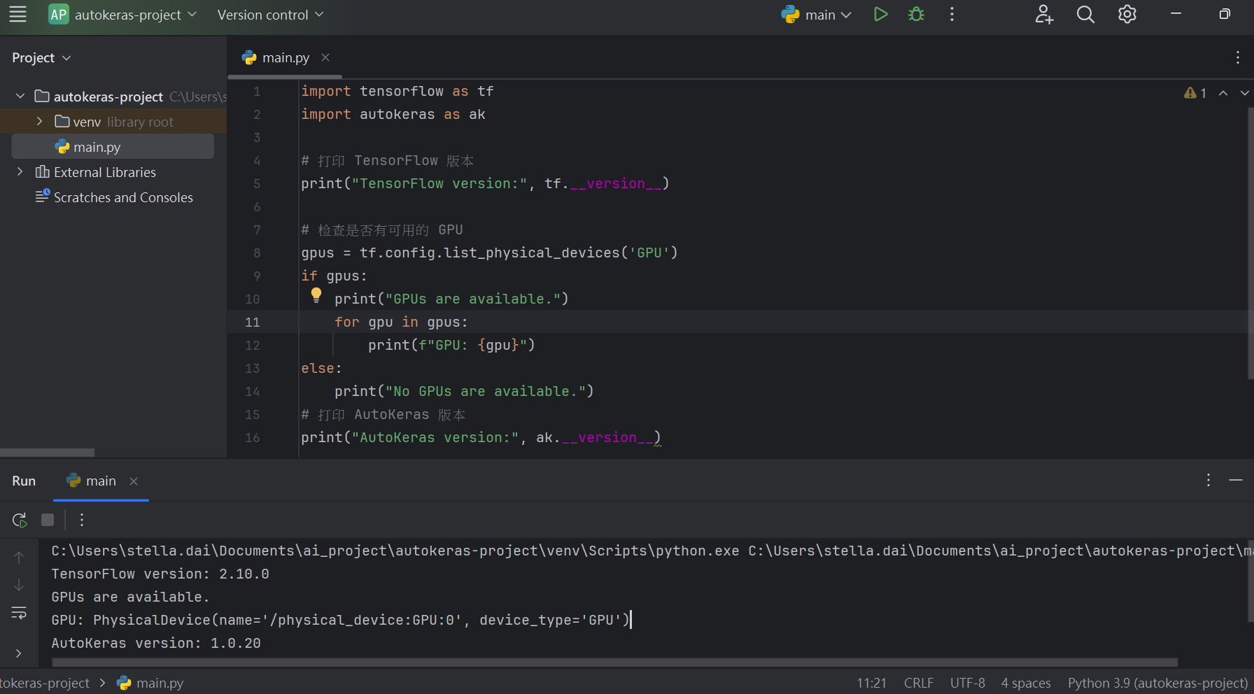
確認 AutoKeras 版本及是否支援 GPU。
1
2
3
4
5
6
7
8
9
10
11
12
13
14
15
16
17
import tensorflow as tfimport autokeras as akprint ("TensorFlow version:" , tf.__version__)gpus = tf.config.list_physical_devices('GPU' ) if gpus: print ("GPUs are available." ) for gpu in gpus: print (f"GPU: {gpu} " ) else : print ("No GPUs are available." ) print ("AutoKeras version:" , ak.__version__)
1
2
3
4
TensorFlow version: 2 .10 .0 GPUs are available.GPU : PhysicalDevice(name='/physical_device:GPU:0 ', device_type='GPU')AutoKeras version: 1 .0 .20
關於如何在本地端啟動 GPU,請看 Win11 本地端啟動 NVIDIA MX450 GPU 的詳細步驟 。
Jupyter Notebook
Conda 建立虛擬環境。
1
2
conda create -n autokeras-env python =3.9 conda activate autokeras-env
安裝 Jupyer Notebook。
安裝 AutoKeras。在 Anaconda 環境下,無法直接安裝 autokeras,會出現 error: subprocess-exited-with-error 錯誤。要使用以下指令安裝autokeras。
1 conda install -c conda-forge auto keras
因為目前安裝 autokeras時,會自動連同 TensorFlow 一起下載,因為我們想要使用 TensorFlow GPU 版本,所以我們需要再安裝 tensorflow-gpu==2.10.0。
1 !pip install tensorflow-gpu ==2.10.0
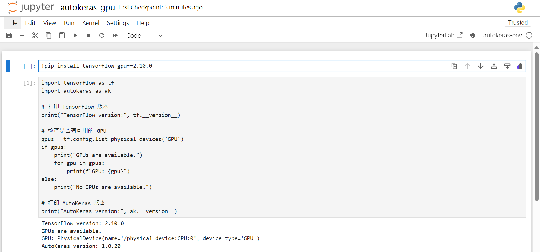
確認 AutoKeras 版本及是否支援 GPU。
1
2
3
4
5
6
7
8
9
10
11
12
13
14
15
16
17
import tensorflow as tfimport autokeras as akprint ("TensorFlow version:" , tf.__version__)gpus = tf.config.list_physical_devices('GPU' ) if gpus: print ("GPUs are available." ) for gpu in gpus: print (f"GPU: {gpu} " ) else : print ("No GPUs are available." ) print ("AutoKeras version:" , ak.__version__)
1
2
3
4
TensorFlow version: 2 .10 .0 GPUs are available.GPU : PhysicalDevice(name='/physical_device:GPU:0 ', device_type='GPU')AutoKeras version: 1 .0 .20
關於如何在本地端啟動 GPU,並使用 Jupyter Notebook 驗證 TensorFlow 是否可用 GPU,請看 Win11 本地端啟動 NVIDIA MX450 GPU 的詳細步驟- 驗證 TensorFlow 可用 GPU 。
Hello MNIST
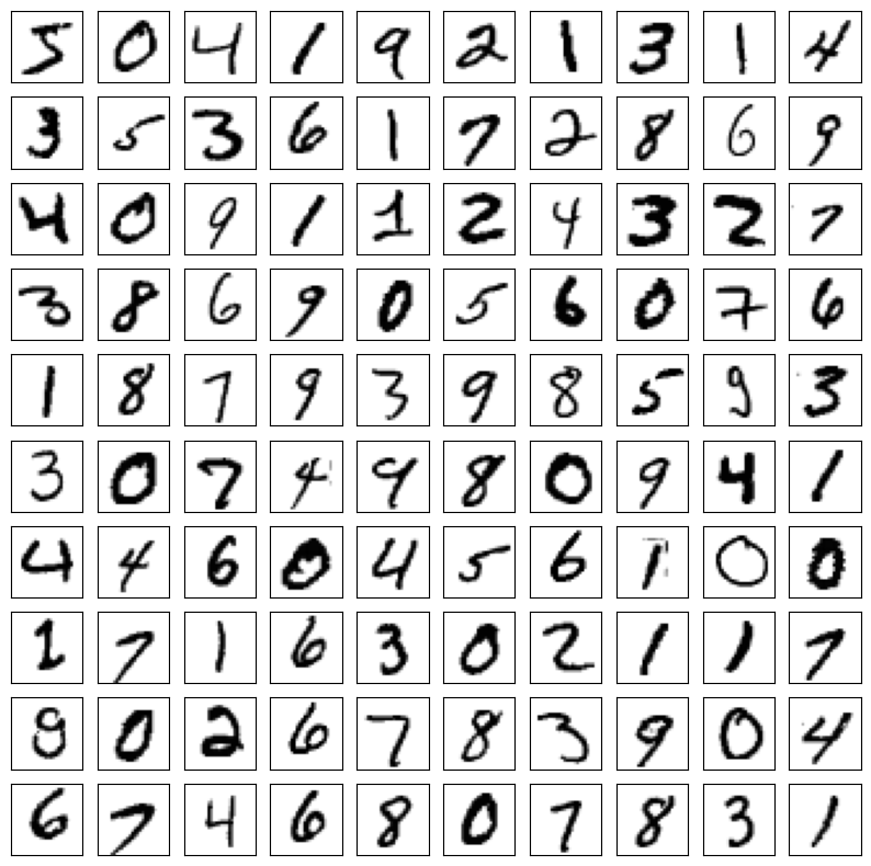
MNIST 是手寫數字(0~9)的圖片的資料集。
由美國國家標準暨技術研究院於 1980 年代收集。
包含 70,000 張圖像,其中 60,000 張訓練圖像和 10,000 張測試圖像。
每張圖像都是 28×28 像素的灰階圖片。
取得 MNIST 資料集
mnist.load_data() 會回傳 x_train、y_train、x_test、y_test 4 個 ndarray 陣列。
資料集
x_train
y_train
x_test
y_test
意義
訓練集資料
訓練集標籤
測試集資料
測試集標籤
1
2
3
4
(x_train, y_train), (x_test, y_test) = mnist.load_data () print (x_train.shape) print (x_test.shape)
1
2
3
4
Downloading data from https:// storage.googleapis.com/tensorflow/ tf-keras-datasets/mnist.npz 11490434 /11490434 ━━━━━━━━━━━━━━━━━━━━ 0s 0us/ step(60000 , 28 , 28 ) (10000 , 28 , 28 )
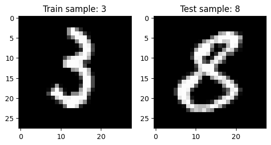
檢視圖像內容
1 2 3 4 5 6 7 8 9 10 11 12 13 14 15 16 17 18 19 fig = plt.figure()ax = fig.add_subplot(1 , 2 , 1 )plt .imshow(x_train[1234 ], cmap='gray')ax .set_title(f'Train sample: {y_train[1234 ]}')ax = fig.add_subplot(1 , 2 , 2 )plt .imshow(x_test[1234 ], cmap='gray')ax .set_title(f'Test sample: {y_test[1234 ]}')plt .show()
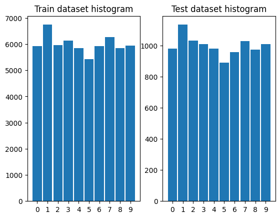
資料分布情況
繪製 MNIST 訓練集和測試集的直方圖。
1 2 3 4 5 6 7 8 9 10 11 12 13 14 15 16 17 18 19 20 21 22 fig = plt.figure()bin = np.arange(11 )ax = fig.add_subplot(1 , 2 , 1 )ax .set_xticks(bin)plt .hist(y_train, bins=bin-0 .5 , rwidth=0 .9 )ax .set_title('Train dataset histogram')ax = fig.add_subplot(1 , 2 , 2 )ax .set_xticks(bin)plt .hist(y_test, bins=bin-0 .5 , rwidth=0 .9 )ax .set_title('Test dataset histogram')plt .show()
看起來 MNIST 訓練集和測試集的資料分布是相近的。
以下我是用 Google Colab 來訓練 MNIST 的圖像分類器和迴歸器。
Hello MNIST: 圖像分類器
準備環境
1 Successfully installed autokeras-2 .0 .0 h5py-3 .11 .0 keras-3 .4 .1 keras-nlp-0 .14 .0 keras-tuner-1 .4 .7 kt-legacy-1 .0 .5 ml-dtypes-0 .3 .2 namex-0 .0 .8 optree-0 .11 .0 tensorboard-2 .16 .2 tensorflow-2 .16 .2 tensorflow-text-2 .16 .1
1
2
3
4
5
import numpy as npimport matplotlib.pyplot as pltimport tensorflow as tffrom tensorflow.keras.datasets import mnistimport autokeras as ak
取得 MNIST 資料集
1 (x_train, y_train), (x_test, y_test) = mnist.load_data()
建置圖像分類器
為了加快訓練時間,將以下參數設定較小。(即便調小,用 Colab CPU 跑也需要跑2小時左右!)
分類器 max_trials 設定只嘗試1種 Keras 模型。
epoch 設定為10個模型訓練週期。
不過實際在進行模型訓練時,應該將以下參數設定較大。
分類器 max_trials (預設為100)。
epochs (預設上限為1000),但可能提前結束。
AutoKeras 發現模型在訓練一段時間後都無法進步的話,也會自動停止訓練。
1 2 3 4 clf = ak.ImageClassifier(max_trials =1) clf.fit(x_train, y_train, epochs =10)
訓練過程中,會輸出目前模型使用的超參數,包含目前表現最佳的模型。
1 2 3 4 5 6 7 8 9 10 11 12 13 14 15 16 17 18 19 20 21 22 23 24 25 26 27 28 29 30 31 32 33 Search : Running Trial #1 Value |Best Value So Far |Hyperparametervanilla |vanilla |image_block_1/block_typeTrue |True |image_block_1/normalizeFalse |False |image_block_1/augment3 |3 |image_block_1/conv_block_1/kernel_size1 |1 |image_block_1/conv_block_1/num_blocks2 |2 |image_block_1/conv_block_1/num_layersTrue |True |image_block_1/conv_block_1/max_poolingFalse |False |image_block_1/conv_block_1/separable0 .25 |0 .25 |image_block_1/conv_block_1/dropout32 |32 |image_block_1/conv_block_1/filters_0_064 |64 |image_block_1/conv_block_1/filters_0_1flatten |flatten |classification_head_1/spatial_reduction_1/reduction_type0 .5 |0 .5 |classification_head_1/dropoutadam |adam |optimizer0 .001 |0 .001 |learning_rateEpoch 1 /10 # 第1 週期訓練1500 /1500 ━━━━━━━━━━━━━━━━━━━━ 13 s 4 ms/step - accuracy: 0 .8984 - loss: 0 .3295 - val_accuracy: 0 .9813 - val_loss: 0 .0660 Epoch 2 /10 1500 /1500 ━━━━━━━━━━━━━━━━━━━━ 6 s 4 ms/step - accuracy: 0 .9744 - loss: 0 .0827 - val_accuracy: 0 .9863 - val_loss: 0 .0491 Epoch 3 /10 1500 /1500 ━━━━━━━━━━━━━━━━━━━━ 5 s 3 ms/step - accuracy: 0 .9797 - loss: 0 .0633 - val_accuracy: 0 .9879 - val_loss: 0 .0466 Epoch 4 /10 1500 /1500 ━━━━━━━━━━━━━━━━━━━━ 6 s 4 ms/step - accuracy: 0 .9830 - loss: 0 .0551 - val_accuracy: 0 .9889 - val_loss: 0 .0418 Epoch 5 /10 1500 /1500 ━━━━━━━━━━━━━━━━━━━━ 5 s 3 ms/step - accuracy: 0 .9854 - loss: 0 .0475 - val_accuracy: 0 .9869 - val_loss: 0 .0442 Epoch 6 /10 1500 /1500 ━━━━━━━━━━━━━━━━━━━━ 6 s 4 ms/step - accuracy: 0 .9866 - loss: 0 .0423 - val_accuracy: 0 .9876 - val_loss: 0 .0460
在訓練過程中,我們可以觀察到4個指標: loss(訓練集損失值)、accuracy(訓練集預測準確率)、val_loss(驗證集損失值)和 val_accuracy(驗證集準確率)。
AutoKeras 會將原始訓練集(60,000 張訓練圖像)自動拆成2個部份:
訓練集: 80%(48,000 筆資料)。
驗證集: 20%(12,000 筆資料)。
AutoKeras 將批次大小設為32,每個週期訓練1500個批次(=48,000/32)。
驗證集在每個週期訓練完後,用於測試模型的泛化能力(Generalization),以評估該週期的訓練效果,或決定是否需要中止訓練。
多數 AutoKeras 模型會嘗試將 val_loss 最小化,驗證集損失值 val_loss 是目前的分類模型訓練的目標指標(objective)。
使用驗證集損失值作為指標,是因為如果訓練集的損失值(loss)持續下降,但驗證集損失值卻上升,這表示模型的泛化能力變差,發生了過擬合(overfitting),此時應該停止訓練。
訓練完成後,則會輸出最佳模型的最終訓練結果。
1
2
3
4
5
6
7
8
9
10
11
12
13
14
15
16
17
18
19
20
21
22
23
24
25
26
27
28
Trial 1 Complete [00h 21m 05s ] val_loss: 0.04181874915957451 Best val_loss So Far: 0.04181874915957451 Total elapsed time: 00h 21m 05s Epoch 1 /10 1875 /1875 ━━━━━━━━━━━━━━━━━━━━ 150s 79ms/step - accuracy: 0.9068 - loss: 0.3083 Epoch 2 /10 1875 /1875 ━━━━━━━━━━━━━━━━━━━━ 144s 77ms/step - accuracy: 0.9761 - loss: 0.0800 Epoch 3 /10 1875 /1875 ━━━━━━━━━━━━━━━━━━━━ 200s 76ms/step - accuracy: 0.9807 - loss: 0.0651 Epoch 4 /10 1875 /1875 ━━━━━━━━━━━━━━━━━━━━ 140s 75ms/step - accuracy: 0.9831 - loss: 0.0543 Epoch 5 /10 1875 /1875 ━━━━━━━━━━━━━━━━━━━━ 141s 75ms/step - accuracy: 0.9859 - loss: 0.0461 Epoch 6 /10 1875 /1875 ━━━━━━━━━━━━━━━━━━━━ 146s 78ms/step - accuracy: 0.9864 - loss: 0.0419 Epoch 7 /10 1875 /1875 ━━━━━━━━━━━━━━━━━━━━ 146s 78ms/step - accuracy: 0.9873 - loss: 0.0383 Epoch 8 /10 1875 /1875 ━━━━━━━━━━━━━━━━━━━━ 142s 76ms/step - accuracy: 0.9885 - loss: 0.0362 Epoch 9 /10 1875 /1875 ━━━━━━━━━━━━━━━━━━━━ 141s 75ms/step - accuracy: 0.9890 - loss: 0.0349 Epoch 10 /10 1875 /1875 ━━━━━━━━━━━━━━━━━━━━ 143s 76ms/step - accuracy: 0.9891 - loss: 0.0327 <keras.src.callbacks.history.History at 0x7bf7b91d4af0 >
AutoKeras 會在所有嘗試過的模型中,自動選擇表現最好的那一個模型,並進行最終的訓練。即最佳模型會再被訓練一次,這次訓練會同時使用訓練集和驗證集的數據 ,這樣可以使模型學到更多的特徵,並產生最終結果。
目前由於 max_trials 參數被設為1,所以唯一一個測試的模型就是最佳模型,因此你會看到這個模型被訓練了2次。這2次差別在於:
第一次訓練時只有訓練集,每個週期訓練1500個批次(=48,000/32)。
第二次已經沒有驗證集,因為 AutoKeras 會合併訓練集和驗證集來做最終的訓練,所以每個週期訓練變成1875個批次(=60000/32)。
若訓練時不指定 epochs 參數,AutoKeras 會記住模型表現最好的那個週期,並在最終訓練時給它訓練同樣次數的週期。
模型對整個原始訓練集的預測準確率達到了 98.91%,以這麼短的訓練時間來說已經很不錯 。
測試集評估模型效能
計算預測準確率
1
2
# 比較測試集的預測分類和實際分類,並傳回預測準確率 clf.evaluate( x_test, y_test)
1
2
313 /313 ━━━━━━━━━━━━━━━━━━━━ 6 s 18 ms/step - accuracy: 0 .9880 - loss: 0 .0413 [0.03329211473464966, 0.9894999861717224]
evaluate() 傳回兩個數值:
第一個是損失值: 0.033
第二個是準確率: 98.94%
我們可以發現模型對測試集的預測準確率為 98.94%,與訓練集的準確率 98.91% 很接近 ,這表示模型沒有發生過擬合(overfitting)問題。
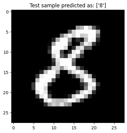
對圖像做出預測
1 2 3 4 5 6 7 8 predicted = clf.predict(x_test[np.newaxis, 1234]) plt.imshow(x_test[1234], cmap ='gray' ) plt.title(f'Test sample predicted as: {predicted[0]}' ) plt.show()
預測結果與真實的標籤值是相符的,代表我們的分類器對這張圖像判斷出了正確結果。
模型視覺化
模型架構表格
1 2 3 4 model = clf.export_model()model .summary()
1
2
3
4
5
6
7
8
9
10
11
12
13
14
15
16
17
18
19
20
21
22
23
24
25
26
27
28
29
30
31
Model : "functional" ┏━━━━━━━━━━━━━━━━━━━━━━━━━━━━━━━━━━━━━━┳━━━━━━━━━━━━━━━━━━━━━━━━━━━━━┳━━━━━━━━━━━━━━━━━┓ ┃ Layer ( type ) ┃ Output Shape ┃ Param # ┃ ┡━━━━━━━━━━━━━━━━━━━━━━━━━━━━━━━━━━━━━━╇━━━━━━━━━━━━━━━━━━━━━━━━━━━━━╇━━━━━━━━━━━━━━━━━┩ │ input_layer ( InputLayer ) │ ( None , 28 , 28 ) │ 0 │ ├──────────────────────────────────────┼─────────────────────────────┼─────────────────┤ │ cast_to _float32 ( CastToFloat32 ) │ ( None , 28 , 28 ) │ 0 │ ├──────────────────────────────────────┼─────────────────────────────┼─────────────────┤ │ expand_last _dim ( ExpandLastDim ) │ ( None , 28 , 28 , 1 ) │ 0 │ ├──────────────────────────────────────┼─────────────────────────────┼─────────────────┤ │ normalization ( Normalization ) │ ( None , 28 , 28 , 1 ) │ 3 │ ├──────────────────────────────────────┼─────────────────────────────┼─────────────────┤ │ conv2d ( Conv2D ) │ ( None , 26 , 26 , 32 ) │ 320 │ ├──────────────────────────────────────┼─────────────────────────────┼─────────────────┤ │ conv2d_ 1 ( Conv2D ) │ ( None , 24 , 24 , 64 ) │ 18 , 496 │ ├──────────────────────────────────────┼─────────────────────────────┼─────────────────┤ │ max_pooling2d ( MaxPooling2D ) │ ( None , 12 , 12 , 64 ) │ 0 │ ├──────────────────────────────────────┼─────────────────────────────┼─────────────────┤ │ dropout ( Dropout ) │ ( None , 12 , 12 , 64 ) │ 0 │ ├──────────────────────────────────────┼─────────────────────────────┼─────────────────┤ │ flatten ( Flatten ) │ ( None , 9216 ) │ 0 │ ├──────────────────────────────────────┼─────────────────────────────┼─────────────────┤ │ dropout_ 1 ( Dropout ) │ ( None , 9216 ) │ 0 │ ├──────────────────────────────────────┼─────────────────────────────┼─────────────────┤ │ dense ( Dense ) │ ( None , 10 ) │ 92 , 170 │ ├──────────────────────────────────────┼─────────────────────────────┼─────────────────┤ │ classification_head _ 1 ( Softmax ) │ ( None , 10 ) │ 0 │ └──────────────────────────────────────┴─────────────────────────────┴─────────────────┘ Total params : 110 , 989 ( 433.55 KB ) Trainable params : 110 , 986 ( 433.54 KB ) Non - trainable params : 3 ( 16.00 B )
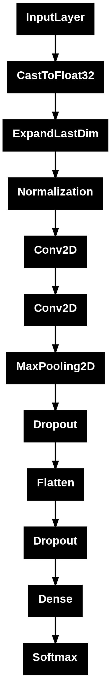
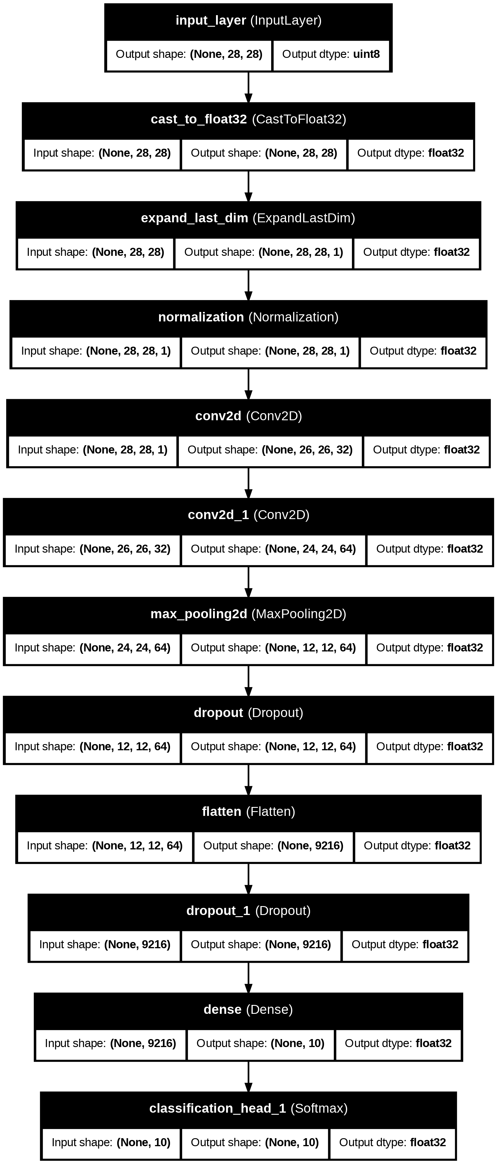
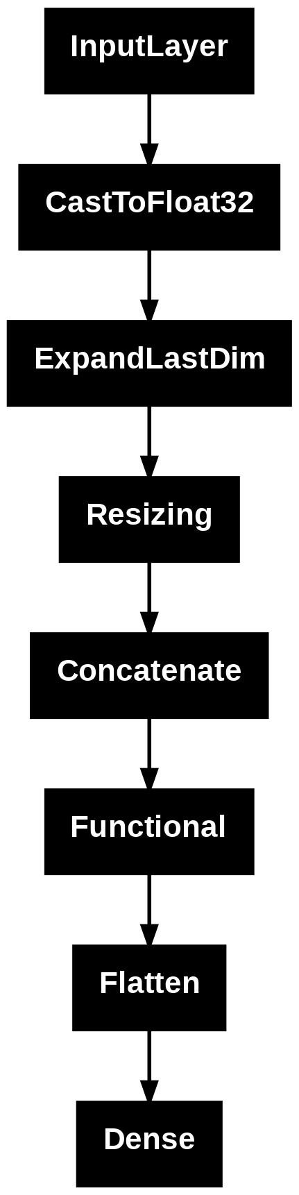
模型架構圖
1
2
from tensorflow.keras .utils import plot_model plot_model (model)
1
2
from tensorflow.keras.utils import plot_modelplot_model(model, to_file ='./mnist_model.png' , show_shapes =True , show_dtype =True , show_layer_names =True )
Hello MNIST: 圖像迴歸器
迴歸器和分類器不同的是,迴歸器會傅回一個貼近預測值的「純量」,比如1.1或8.9,而非絕對的 0~9 整數 。在此為了預測數字,會將預測值四捨五入,看看它最接近哪個整數,並將之視為最終預測結果。
準備環境
1 Successfully installed autokeras-2 .0 .0 h5py-3 .11 .0 keras-3 .4 .1 keras-nlp-0 .14 .0 keras-tuner-1 .4 .7 kt-legacy-1 .0 .5 ml-dtypes-0 .3 .2 namex-0 .0 .8 optree-0 .11 .0 tensorboard-2 .16 .2 tensorflow-2 .16 .2 tensorflow-text-2 .16 .1
1
2
3
4
import matplotlib.pyplot as pltimport tensorflow as tffrom tensorflow.keras.datasets import mnistimport autokeras as ak
取得 MNIST 資料集
1 (x_train, y_train), (x_test, y_test) = mnist.load_data()
建置圖像迴歸器
1
2
reg = ak.ImageRegressor(overwrite =True , max_trials =1) reg.fit(x_train, y_train, epochs =20)
訓練過程中,會輸出目前模型使用的超參數,包含目前表現最佳的模型。
1
2
3
4
5
6
7
8
9
10
11
12
13
14
15
16
17
18
19
20
21
22
23
24
25
26
27
28
29
Search : Running Trial #1 Value |Best Value So Far |HyperparameterFalse |False |image_block_1/normalizeFalse |False |image_block_1/augmentresnet |resnet |image_block_1/block_typeFalse |False |image_block_1/res_net_block_1/pretrainedresnet50 |resnet50 |image_block_1/res_net_block_1/versionFalse |False |image_block_1/res_net_block_1/imagenet_size0 |0 |regression_head_1/dropoutadam |adam |optimizer0 .001 |0 .001 |learning_rateEpoch 1 /20 1500 /1500 ━━━━━━━━━━━━━━━━━━━━ 122 s 36 ms/step - loss: 4 .0871 - mean_squared_error: 4 .0871 - val_loss: 1 .1759 - val_mean_squared_error: 1 .1759 Epoch 2 /20 1500 /1500 ━━━━━━━━━━━━━━━━━━━━ 50 s 33 ms/step - loss: 0 .6240 - mean_squared_error: 0 .6240 - val_loss: 0 .4633 - val_mean_squared_error: 0 .4633 Epoch 3 /20 1500 /1500 ━━━━━━━━━━━━━━━━━━━━ 48 s 32 ms/step - loss: 0 .5289 - mean_squared_error: 0 .5289 - val_loss: 0 .5131 - val_mean_squared_error: 0 .5131 Epoch 4 /20 1500 /1500 ━━━━━━━━━━━━━━━━━━━━ 56 s 37 ms/step - loss: 0 .4572 - mean_squared_error: 0 .4572 - val_loss: 0 .3757 - val_mean_squared_error: 0 .3757 Epoch 5 /20 1500 /1500 ━━━━━━━━━━━━━━━━━━━━ 48 s 32 ms/step - loss: 0 .4649 - mean_squared_error: 0 .4649 - val_loss: 0 .8890 - val_mean_squared_error: 0 .8890 Epoch 6 /20 1500 /1500 ━━━━━━━━━━━━━━━━━━━━ 48 s 32 ms/step - loss: 0 .4681 - mean_squared_error: 0 .4681 - val_loss: 0 .4839 - val_mean_squared_error: 0 .4839 Epoch 7 /20 1500 /1500 ━━━━━━━━━━━━━━━━━━━━ 47 s 31 ms/step - loss: 0 .6746 - mean_squared_error: 0 .6746 - val_loss: 2 .2674 - val_mean_squared_error: 2 .2674 Epoch 8 /20 1500 /1500 ━━━━━━━━━━━━━━━━━━━━ 48 s 32 ms/step - loss: 0 .3672 - mean_squared_error: 0 .3672 - val_loss: 3 .1101 - val_mean_squared_error: 3 .1101
訓練完成後,則會輸出最佳模型的最終訓練結果。
1
2
3
4
5
6
7
8
9
10
11
12
13
14
15
16
17
18
19
20
21
22
23
24
25
26
27
28
29
30
31
32
33
34
35
36
37
38
39
40
41
42
43
44
45
46
Trial 1 Complete [00h 18m 25s] val_loss : 0 .17454160749912262 Best val_loss So Far: 0 .17454160749912262 Total elapsed time: 00 h 18 m 25 sEpoch 1 /20 1875 /1875 ━━━━━━━━━━━━━━━━━━━━ 118 s 31 ms/step - loss: 3 .3630 - mean_squared_error: 3 .3630 Epoch 2 /20 1875 /1875 ━━━━━━━━━━━━━━━━━━━━ 58 s 31 ms/step - loss: 0 .5886 - mean_squared_error: 0 .5886 Epoch 3 /20 1875 /1875 ━━━━━━━━━━━━━━━━━━━━ 58 s 31 ms/step - loss: 0 .5281 - mean_squared_error: 0 .5281 Epoch 4 /20 1875 /1875 ━━━━━━━━━━━━━━━━━━━━ 82 s 31 ms/step - loss: 0 .4323 - mean_squared_error: 0 .4323 Epoch 5 /20 1875 /1875 ━━━━━━━━━━━━━━━━━━━━ 57 s 30 ms/step - loss: 0 .5396 - mean_squared_error: 0 .5396 Epoch 6 /20 1875 /1875 ━━━━━━━━━━━━━━━━━━━━ 58 s 31 ms/step - loss: 0 .3970 - mean_squared_error: 0 .3970 Epoch 7 /20 1875 /1875 ━━━━━━━━━━━━━━━━━━━━ 58 s 31 ms/step - loss: 0 .4000 - mean_squared_error: 0 .4000 Epoch 8 /20 1875 /1875 ━━━━━━━━━━━━━━━━━━━━ 82 s 31 ms/step - loss: 0 .3490 - mean_squared_error: 0 .3490 Epoch 9 /20 1875 /1875 ━━━━━━━━━━━━━━━━━━━━ 57 s 31 ms/step - loss: 0 .2903 - mean_squared_error: 0 .2903 Epoch 10 /20 1875 /1875 ━━━━━━━━━━━━━━━━━━━━ 84 s 32 ms/step - loss: 0 .2293 - mean_squared_error: 0 .2293 Epoch 11 /20 1875 /1875 ━━━━━━━━━━━━━━━━━━━━ 58 s 31 ms/step - loss: 0 .2057 - mean_squared_error: 0 .2057 Epoch 12 /20 1875 /1875 ━━━━━━━━━━━━━━━━━━━━ 58 s 31 ms/step - loss: 0 .1904 - mean_squared_error: 0 .1904 Epoch 13 /20 1875 /1875 ━━━━━━━━━━━━━━━━━━━━ 84 s 32 ms/step - loss: 0 .1911 - mean_squared_error: 0 .1911 Epoch 14 /20 1875 /1875 ━━━━━━━━━━━━━━━━━━━━ 58 s 31 ms/step - loss: 0 .1596 - mean_squared_error: 0 .1596 Epoch 15 /20 1875 /1875 ━━━━━━━━━━━━━━━━━━━━ 82 s 31 ms/step - loss: 0 .1527 - mean_squared_error: 0 .1527 Epoch 16 /20 1875 /1875 ━━━━━━━━━━━━━━━━━━━━ 57 s 31 ms/step - loss: 0 .1361 - mean_squared_error: 0 .1361 Epoch 17 /20 1875 /1875 ━━━━━━━━━━━━━━━━━━━━ 57 s 31 ms/step - loss: 0 .1056 - mean_squared_error: 0 .1056 Epoch 18 /20 1875 /1875 ━━━━━━━━━━━━━━━━━━━━ 57 s 31 ms/step - loss: 0 .0992 - mean_squared_error: 0 .0992 Epoch 19 /20 1875 /1875 ━━━━━━━━━━━━━━━━━━━━ 59 s 31 ms/step - loss: 0 .1010 - mean_squared_error: 0 .1010 Epoch 20 /20 1875 /1875 ━━━━━━━━━━━━━━━━━━━━ 58 s 31 ms/step - loss: 0 .0957 - mean_squared_error: 0 .0957 <keras.src.callbacks.history.History at 0x7ef7602e47f0>
模型訓練時,模型會更新權重,並試著讓均方誤差(Mean Square Error, MSE)最小化。
我們最終得到的 MSE 為 0.0957,其平方根即為均方根誤差(RMSE)為 0.3094 。RMSE 為 0.3094,表示平均每個預測值與真實值之間的差距約為 0.3094,也就是指此模型的平均預測誤差約為 0.3094。
均方誤差(mean square error, MSE),表示預測值與真實值之間的差距,是所有預測值與真實值的差距的平方和的平均值。通常一個較小的 MSE 或 RMSE 表示模型的預測精度較高。關於機器學習迴歸模型中常見的的效能衡量指標,請看 機器學習中迴歸模型的效能衡量指標 這篇文章。
測試集評估模型效能
計算均方誤差
1 print (reg.evaluate(x_test, y_test)
1
2
313 /313 ━━━━━━━━━━━━━━━━━━━━ 11 s 15 ms/step - loss: 0 .1685 - mean_squared_error: 0 .1685 [0.1497689187526703, 0.1497689187526703]
我們可以發現,模型在測試集上的預測均方誤差(MSE)為 0.1498,其均方根誤差(RMSE)約為 0.387。
對圖像做出預測
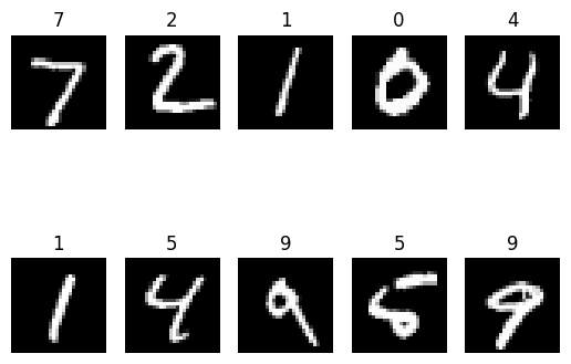
1 2 3 4 5 6 7 8 9 10 11 12 13 14 15 16 17 predicted = reg.predict(x_test[:10 ]).flatten().round().astype('uint8')print (y_test[:10 ])print (predicted)fig = plt.figure()for i in range(10 ): ax = fig.add_subplot(2 , 5 , i + 1 ) ax .set_axis_off() plt .imshow(x_test[i], cmap='gray') ax .set_title(predicted[i]) plt .show()
1
2
3
4
1/1 ━━━━━━━━━━━━━━━━━━━━ 5s 5s/step 1/1 ━━━━━━━━━━━━━━━━━━━━ 0s 9ms/step [7 2 1 0 4 1 4 9 5 9] [7 2 1 0 4 1 5 9 5 9]
可見儘管迴歸器的預測值不是整數,但只要訓練時得到的均方誤差(MSE)夠小,四捨五入後還是能貼近真實標籤。不過一般來說,迴歸模型的用途大多還是用在預測非離散的數值,例如房價等。
模型視覺化
模型架構表格
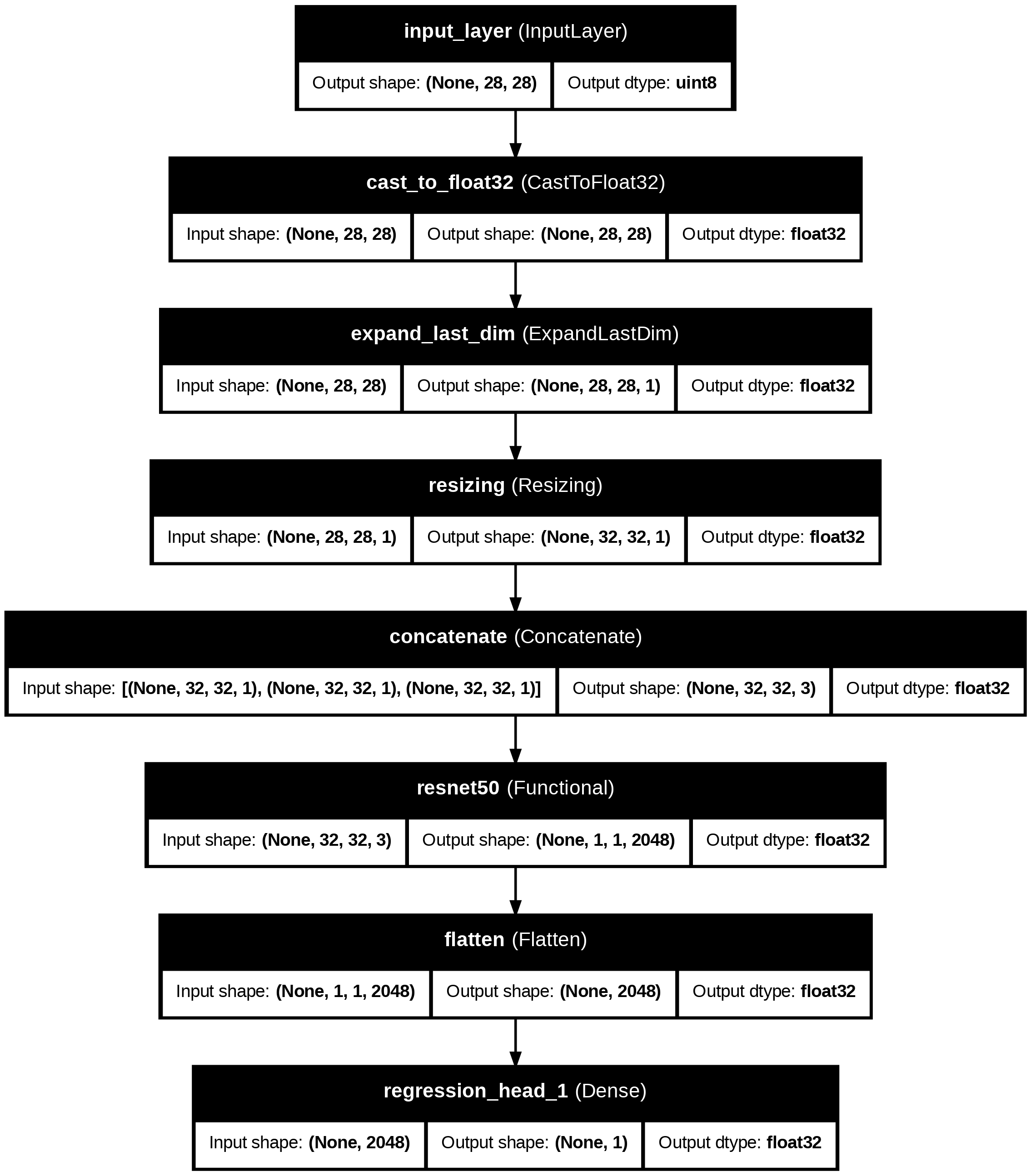
1
2
model = reg.export_model()model.summary()
1
2
3
4
5
6
7
8
9
10
11
12
13
14
15
16
17
18
19
20
21
22
23
24
25
26
27
Model : "functional" ┏━━━━━━━━━━━━━━━━━━━━━━━━━━━┳━━━━━━━━━━━━━━━━━━━━━━━━┳━━━━━━━━━━━━━━━━┳━━━━━━━━━━━━━━━━━━━━━━━━┓ ┃ Layer (type) ┃ Output Shape ┃ Param # ┃ Connected to ┃ ┡━━━━━━━━━━━━━━━━━━━━━━━━━━━╇━━━━━━━━━━━━━━━━━━━━━━━━╇━━━━━━━━━━━━━━━━╇━━━━━━━━━━━━━━━━━━━━━━━━┩ │ input_layer (InputLayer ) │ (None , 28 , 28 ) │ 0 │ - │ ├───────────────────────────┼────────────────────────┼────────────────┼────────────────────────┤ │ cast_to_float32 │ (None , 28 , 28 ) │ 0 │ input_layer[0 ][0 ] │ │ (CastToFloat32 ) │ │ │ │ ├───────────────────────────┼────────────────────────┼────────────────┼────────────────────────┤ │ expand_last_dim │ (None , 28 , 28 , 1 ) │ 0 │ cast_to_float32[0 ][0 ] │ │ (ExpandLastDim ) │ │ │ │ ├───────────────────────────┼────────────────────────┼────────────────┼────────────────────────┤ │ resizing (Resizing ) │ (None , 32 , 32 , 1 ) │ 0 │ expand_last_dim[0 ][0 ] │ ├───────────────────────────┼────────────────────────┼────────────────┼────────────────────────┤ │ concatenate (Concatenate ) │ (None , 32 , 32 , 3 ) │ 0 │ resizing[0 ][0 ], │ │ │ │ │ resizing[0 ][0 ], │ │ │ │ │ resizing[0 ][0 ] │ ├───────────────────────────┼────────────────────────┼────────────────┼────────────────────────┤ │ resnet50 (Functional ) │ (None , 1 , 1 , 2048 ) │ 23 ,587 ,712 │ concatenate[0 ][0 ] │ ├───────────────────────────┼────────────────────────┼────────────────┼────────────────────────┤ │ flatten (Flatten ) │ (None , 2048 ) │ 0 │ resnet50[0 ][0 ] │ ├───────────────────────────┼────────────────────────┼────────────────┼────────────────────────┤ │ regression_head_1 (Dense ) │ (None , 1 ) │ 2 ,049 │ flatten[0 ][0 ] │ └───────────────────────────┴────────────────────────┴────────────────┴────────────────────────┘ Total params: 23 ,589 ,761 (89.99 MB ) Trainable params: 23 ,536 ,641 (89.79 MB ) Non -trainable params: 53 ,120 (207.50 KB )
模型架構圖
1
2
from tensorflow.keras .utils import plot_model plot_model (model)
1
2
from tensorflow.keras.utils import plot_modelplot_model(model, to_file ='./mnist_model.png' , show_shapes =True , show_dtype =True , show_layer_names =True )
總結
本篇文章詳細介紹了如何在不同環境下如何安裝 AutoKeras,並使用 AutoKeras 來訓練 MNIST 的圖像分類器和迴歸器,從環境配置、資料集準備、模型訓練到最終評估,逐步展示了每個過程的詳細步驟。
AutoKeras 框架讓我們實現短短幾行程式碼下,就能針對手寫數字圖像實作出高預測精確度的圖像分類器和迴歸器模型。關於如何準備資料集,請看 【AutoKeras】準備資料集及資料夾結構 這篇文章。